Week 03 - Lecture Part 1
Representation Models: Methods and Techniques
Representation Models
So what are representation models and why are they important? Representation models help us plan our geodesign project and relate it to the geographic context of the area being studied. As mentioned, in the introduction geography matters, it provides us with the relevant context in framing our design problems, issues, goals, and objectives that we discussed last week. There are several components to geography: scale and size.
Scale refers to the lens through which we will look at our study area, including the level of detail we choose to consider or ignore. In landscape architecture, planning, and geodesign a larger scale means a closer more detailed view. This has also been referred to as high resolution, specifically when speaking of high-resolution data. In other words at what scale should we design: site, neighborhood, municipal, regionally, nationally, global? Should we work at all levels simultaneously? Carl Steinitz, A framework for geodesign: changing geography by design, illustrates the principles of scale very well in Chapter 2 of your readings for this course. Think about the principles of scale and how they impact your work.
Using this Padlet answer the question: List a project you have or are currently working on and briefly explain how different scales of thinking, data, or problem definition would impact how you proceed(ed) on this project.
Additionally, size matters. Carl Steinitz also does a great job of describing how size matters (Steinitz, 2012). The size of the study area is important because as size of the area increases so do scientific complexity and the level of risk for harmful impact if you make a mistake. Also, as the size increases the publics knowledge and understanding decreases. It is because of this that we must be meticulous in our planning, communication, and choices of methods. For example, if a single building uses a material or style we do not like, it really does not negatively impact our daily lives. However, if all buildings in a city use copper roofs and walls, thus causing heavy metal pollution of the regional drinking water supply, it is a very important risk. As these risks increase serious scientific information and robust documentation and analyses are needed.
Another example: if we are designing a garden space for a home owner we can probably get away with a few site visits, hand produced, surveyed base maps and little else in terms of data or analyses. Even from this level of data collection we can see evidence if a house sites in the floodplain. However, if we are working regionally on watershed issues we need complex datasets and analyses to see how hydrology works across the regions, the number of people and amount of infrastructure that are impacted by the floodplain. Additionally, we need to understand the interplay between a variety of systems. The more complicated the problem and processes the need for rigorous documentation, communication, and analyses need to be, to ensure public safety, allow further testing and critique, and ensure that we are using the most effective and appropriate data and methods. Hence, the imperative nature of the first two steps in the geodesign process.
Representation models help frame the geographic context and systems with which we are dealing. During this step of the process we seek to answer the following questions:
- Where is the study area?
- How should it be defined?
- What are its physical, ecological, economic, and social geographies?
- What are its physical, ecological, economic, and social histories?
Types of Representation Models
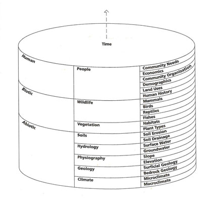
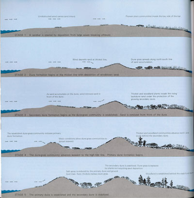
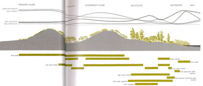
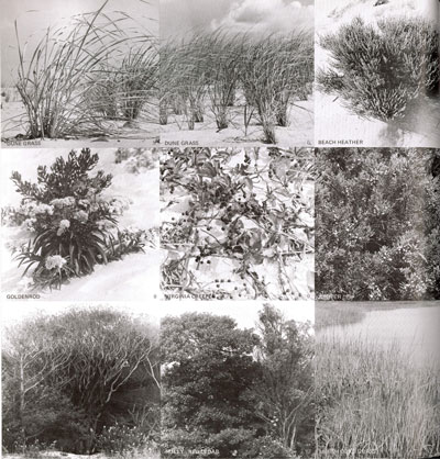
Ian McHarg is well known for his layer-cake model for inventorying human, biotic, and abiotic systems (Steiner, 2008). This model came from Ian McHarg’s belief that “many of the problems that society confronts are of such inordinate complexity that it takes the greatest of dedication and seal to assemble the necessary data, analyze, and prescribe” (McHarg, 1992, p. 7). As a result, McHarg created a systematic method for thinking about the data needed to answer these questions. Although, to internalize, process, and communicate these ideas and principles he also relied on several methods: diagrams, maps, and other graphic elements to compile a representation of the projects geographic context. However, his techniques and methods were driven by the overall layer-cake model plan.
Click on the below images to view a larger version in a new tab.

Photo credit: Layer-cake model, source: (Steiner, 2008) |

Photo credit: Dune section typologies, source: (McHarg, 1992) |

Photo credit: Dune community types, source: (McHarg, 1992) |

Photo credit: Plant images, source: (McHarg, 1992) |
Steinitz, Steiner, and others built off of McHarg’s work, adding further information that is necessary to complete geodesign projects at various scales. From McHarg’s work an adapted baseline of natural resources has been compiled. This list of resources is deemed necessary for ecological planning and geodesign. This list includes broad groups of climate, geology, surficial geology, groundwater hydrology, physiography, surficial hydrology, soils, vegetation, wildlife, and human systems. Table 1 shows further details of these requirements. Table 2 and 3 contain other forms of data or information classification depending on the context of the project. Table 3 is unique to the method of remote sensing, a method for data collection at a wide range of scales: watershed, regional, national, and world scale. However, without a rigorously defined classification scale the data would be meaningless.
| Table 1: Baseline Nature Resource Inventory |
|---|
| Climate: temperature, humidity, precipitation, wind velocity, wind direction, wind duration, first and last frosts, snow, frost, fog, inversions, hurricanes, tornadoes, tsunamis, typhoons, and Chinook winds |
| Geology: rocks, ages, formations, plans, sections, properties, seismic activity, earthquakes, rock slides, mud slides, and subsidence (e.g. sinkholes, etc) |
| Surficial Geology: kames, kettles, eskers, moraines, drift and till |
| Groundwater Hydrology: geological formations interpreted as aquifers with well locations, well logs, water quantity and quality, and water table |
| Physiography: physiographic regions, subregions, features, contours, sections, slopes, aspect, insolation, and digital terrain models |
| Surficial Hydrology: oceans, lakes deltas, rivers, streams, creeks, marshes, swamps, wetlands, stream orders, density, discharges, gauges, water quality, and floodplains |
| Soils: soil associations, soil series, properties, depth to seasonal high water table, depth to bedrock, shrink-swell, compressive strength, cation and anion exchange, and acidity-alkalinity |
| Vegetation: associations, communities, species, composition, distribution, age and condition, visual quality, species number, rare and endangered species, fire history, and successional history |
| Wildlife: habitats, animal populations, census data, rare and endangered species, and scientific and educational value |
| Human: ethnographic history, settlement patterns, existing land use, existing infrastructure, economic activities, population characteristics |
Several other ‘checklists’ of data needs exist, in many cases they are expansions of McHarg’s list above; however, their differences are important. I will present them below, as the will help you determine your own data needs for your representation model plans.
| Table 2: UNESCO Total Environmental Checklist: Components and Processes |
|---|
| Natural Environment – Components: soil, water, atmosphere, mineral resources, energy resources, fauna, flora, and microorganisms |
| Natural Environment – Process: biogeochemical cycles, irradiation, climatic processes, photosynthesis, animal and plant growth, fluctuations in animal and plant growth, changes in fertility, salinity, and alkalinity, host/parasite interactions, and epidemic processes |
| Human Population – Demographic Aspects: Population structure (age, ethnicity, economic, education, and occupation), population size, population density, fertility and mortality rates, and health statistics |
| Human Activities and the Use of Machines: migratory movements, daily mobility, decision making, mining, industrial activities, commercial activities, exercise and distribution of authority, administration, farming, fishing, military activities, transportation, recreational activities, and crime rates |
| Societal Groupings: governmental groupings, industrial groupings, commercial groupings, political groupings, religious groupings, educational groupings, information media, law-keeping, health services, community groupings, and family groupings |
| Products of Labor: built environment (buildings, roads, railways, and parks), food, pharmaceutical products, machines, and other commodities |
| Culture: values, beliefs, attitudes, knowledge, information, technology, literature, laws, and economic system |
| Table 3: United State Geological Survey Land-Use and Land-Cover Classification System | |
|---|---|
| Level I | Level II |
| 1 – Urban or built-up land | 11 – Residential 12 – Commercial and services 13 – Industrial 14 – Transportation, communications and services 15 – Industrial and commercial complexes 16 – Mixed urban or built-up land 17 – Other urban or built-up land |
| 2 – Agricultural Land | 21 – Cropland and pasture 22 – Orchards, groves, vineyards, nurseries, and ornamental horticulture 23 – Confined feeding operations 24 – Other agricultural land |
| 3 – Rangeland | 31 – Herbaceous rangeland 32 – Shrub and brush rangeland 33 – Mixed rangeland |
| 4 – Forestland | 41 – Deciduous forestland 42 – Evergreen forestland 43 – Mixed forestland |
| 5 – Water | 51 – Streams and canals 52 – Lakes 53 – Reservoirs 54 – Bays and estuaries |
| 6 – Wetland | 61 – Forested wetland 62 – Nonforested wetland |
| 7 – Barren land | 71 – Dry salt flats 72 – Beaches 73 – Sandy areas other than beaches 74 – Bare exposed rocks 75 – Strip mines, quarries, and gravel pits 76 – Transitional areas 77 – Mixed barren land |
| 8 – Tundra | 81 – Shrub and brush tundra 82 – Herbaceous tundra 83 – Bare ground 84 – Mixed tundra |
| 9 – Perennial snow ice | 91 – Perennial snowfields 92 - Glaciers |
These data categories and classification structure examples reinforce the need to have a plan for what and how we are representing our projects geography. These examples also have inherent scales attached to them, for example looking at Table 3, we have two levels of land-cover classification: a broad category (Level I) and a more refined category (Level II).
Using this Padlet answer the question: In what circumstance might you need to augment the number of levels obtained from satellite data?
Now that the needs for our plan are taking shape, lets move on to the types of data we can collect and how we go about representing our data.